Physical quantity
A physical quantity is a physical property of a phenomenon, body, or substance, that can be quantified by measurement.[1]
Definition of a physical quantity
Formally, the International Vocabulary of Metrology, 3rd edition (VIM3) defines quantity as:
Property of a phenomenon, body, or substance, where the property has a magnitude that can be expressed as a number and a reference.[2]
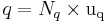
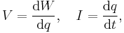
Hence the value of a physical quantity q is expressed as the product of a numerical value Nq and a unit of measurement uq;
Quantity calculus describes how to do maths with quantities.
Examples
- If the temperature T of a body is quantified as 300 kelvin (in which T is the quantity symbol, 300 the value, and K is the unit), this is written
- T = 300 × K = 300 K,
- If a person weighs 120 pounds, then "120" is the numerical value and "pound" is the unit. This physical quantity mass would be written as "120 lb", or
- m = 120 lb
- If a person traveling with a yardstick, measures the length of such yardstick, the physical quantity of length would be written as
- L = 36 inches
- An example employing SI units and scientific notation for the number, might be a measurement of power written as
- P = 42.3 × 10³ W,
In practice, note that different observers may get different values of a quantity depending on the frame of reference; in turn the coordinate system and metric. Physical properties such as length, mass or time, by themselves, are not physically invariant. However, the laws of physics which include these properties are invariant.
Extensive and intensive quantities
Extensive quantity: its magnitude is additive for subsystems (volume, mass, etc.)
Intensive quantity: the magnitude is independent of the extent of the system (temperature, pressure, etc.)
There are also physical quantities that can be classified as neither extensive nor intensive, for example angular momentum, area, force, length, and time.
Symbols, nomenclature
General: Symbols for quantities should be chosen according to the international recommendations from ISO 80000, the IUPAP red book and the IUPAC green book. For example, the recommended symbol for the physical quantity 'mass' is m, and the recommended symbol for the quantity 'charge' is Q.
Subscripts and indices
Subscripts are used for two reasons, to simply attach a name to the quantity or associate it with another quantity, or represent a specific vector, matrix, or tensor component.
- Name reference: The quantity has a subscripted or superscripted single letter, a number of letters, or an entire word, to specify what concept or entity they refer to, and tend to be written in upright roman typeface rather than italic while the quantity is in italic. For instance Ek or Ekinetic is usually used to denote kinetic energy and Ep or Epotential is usually used to denote potential energy.
- Quantity reference: The quantity has a subscripted or superscripted single letter, a number of letters, or an entire word, to specify what measurement/s they refer to, and tend to be written in italic rather than upright roman typeface while the quantity is also in italic. For example cp or cisobaric is heat capacity at constant pressure.
- Note the difference in the style of the subscripts: k and p are abbreviations of the words kinetic and potential, whereas p (italic) is the symbol for the physical quantity pressure rather than an abbreviation of the word "pressure".
- Indices: These are quite apart from the above, their use is for mathematical formalism, see Index notation.
Scalars: Symbols for physical quantities are usually chosen to be a single letter of the Latin or Greek alphabet, and are printed in italic type.
Vectors: Symbols for physical quantities that are vectors are in bold type, underlined or with an arrow above. If, e.g., u is the speed of a particle, then the straightforward notation for its velocity is u, u, or  .
.
Numbers and elementary functions
Numerical quantities, even those denoted by letters, are usually printed in roman (upright) type, though sometimes can be italic. Symbols for elementary functions (circular trigonometric, hyperbolic, logarithmic etc.), changes in a quantity like Δ in Δy or operators like d in dx, are also recommended to be printed in roman type.
- Examples
- real numbers are as usual, such as 1 or √2,
- e for the base of natural logarithm,
- i for the imaginary unit,
- π for 3.14152658...
- δx, Δy, dz,
- sin α, sinh γ, log x
Units and dimensions
Units
Most physical quantities include a unit, but not all - some are dimensionless. Neither the name of a physical quantity, nor the symbol used to denote it, implies a particular choice of unit, though SI units are usually preferred and assumed today due to their ease of use and all-round applicability. For example, a quantity of mass might be represented by the symbol m, and could be expressed in the units kilograms (kg), pounds (lb), or Daltons (Da).
Dimensions
The notion of physical dimension of a physical quantity was introduced by Joseph Fourier in 1822.[3] By convention, physical quantities are organized in a dimensional system built upon base quantities, each of which is regarded as having its own dimension.
Base quantities
Base quantities
The seven base quantities of the International System of Quantities (ISQ) and their corresponding SI units and dimensions are listed in the following table. Other conventions may have a different number of fundamental units (e.g. the CGS and MKS systems of units).
| Quantity name/s | (Common) Quantity symbol/s | SI unit name | SI unit symbol | Dimension symbol |
|---|---|---|---|---|
| Length, width, height, depth | a, b, c, d, h, l, r, w, x, y, z | metre | m | [L] |
| Time | t | second | s | [T] |
| Mass | m | kilogram | kg | [M] |
| Temperature | T, θ | kelvin | K | [Θ] |
| Amount of substance, number of moles | n | mole | mol | [N] |
| Electric current | i, I | ampere | A | [I] |
| Luminous intensity | Iv | candela | Cd | [J] |
| Plane angle | α, β, γ, θ, φ, χ | radian | rad | dimensionless |
| Solid angle | ω, Ω | steradian | sr | dimensionless |
The last two angular units; plane angle and solid angle are subsidiary units used in the SI, but treated dimensionless. The subsidiary units are used for convenience to differentiate between a truly dimensionless quantity (pure number) and an angle, which are different measurements.
Physical quantities defined from equations
Description of units and physical quantities
Physical quantities and units follow the same hierarchy; chosen base quantities have defined base units, from these any other quantities may be derived and have corresponding derived units.
Colour mixing analogy
Defining quantities is analogous to mixing colours, and could be classified a similar way, although this is not standard. Primary colours are to base quantities; as secondary (or tertiary etc.) colours are to derived quantities. Mixing colours is analogous to combining quantities using mathematical operations. But colours could be for light or paint, and analogously the system of units could be one of many forms: such as SI (now most common), CGS, Gaussian, old imperial units, a specific form of natural units or even arbitrarily defined units characteristic to the physical system in consideration (characteristic units).
The choice of a base system of quantities and units is arbitrary; but once chosen it must be adhered to throughout all analysis which follows for consistency. It makes no sense to mix up different systems of units. Choosing a system of units, one system out of the SI, CGS etc., is like choosing whether use paint or light colours.
In light of this analogy, primary definitions are base quantities with no defining equation, but defined standardized condition, "secondary" definitions are quantities defined purely in terms of base quantities, "tertiary" for quantities in terms of both base and "secondary" quantities, "quaternary" for quantities in terms of base, "secondary", and "tertiary" quantities, and so on.
Motivation
Much of physics requires definitions to be made for the equations to make sense.
Theoretical implications: Definitions are important since they can lead into new insights of a branch of physics. Two such examples occurred in classical physics. When entropy S was defined – the range of thermodynamics was greatly extended by associating chaos and disorder with a numerical quantity that could relate to energy and temperature, leading to the understanding of the second thermodynamic law and statistical mechanics. Also the action functional (also written S) (together with generalized coordinates and momenta and the lagrangian function), initially an alternative formulation of classical mechanics to Newton's laws, now extends the range of modern physics in general – notably quantum mechanics and particle physics.
Analytical convenience: They allow other equations to be written more compactly and so allow easier mathematical manipulation; by including a parameter in a definition, occurrences of the parameter can be absorbed into the substituted quantity and removed from the equation.
- Example
- As an example consider Ampère's circuital law (with Maxwell's correction) in integral form for an arbitrary current carrying conductor in a vacuum (so zero magnetization due medium, i.e M = 0):
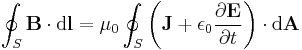
- using the constitutive definition

- and the current density definition
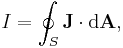
- similarly for the displacement current density
 leading to the displacement current
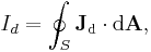
- we have
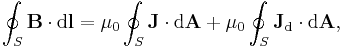
- which is simpler to write, even if the equation is the same.
Ease of comparison: They allow comparisons of measurements to be made when they might appear ambiguous and unclear otherwise.
- Example
- A basic example is mass density. It is not clear how compare how much matter constitutes a variety of substances given only their masses or only their volumes. Given both for each substance, the mass m per unit volume V, or mass density ρ provides a meaningful comparison between the substances, since for each, a fixed amount of volume will correspond to an amount of mass depending on the substance. To illustrate this; if two substances A and B have masses mA and mB respectively, occupying volumes VA and VB respectively, using the definition of mass density gives:
- ρA = mA / VA , ρB = mB / VB
- following this can be seen that:
- if mA > mB or mA < mB and VA = VB, then ρA > ρB or ρA < ρB,
- if mA = mB and VA > VB or VA < VB, then ρA < ρB or ρA > ρB,
- if ρA = ρB, then ρA > ρB, then mA / VA = mB / VB so mA / mB = VA / VB, demonstrating that if mA > mB or mA < mB, then VA > VB or VA < VB.
Construction of defining equations
Scope of defining equations
Defining equations are normally formulated in terms of elementary algebra and calculus, vector algebra and calculus, or for the most general applications tensor algebra and calculus, depending on the level of study and presentation, complexity of topic and scope of applicability. Functions may be incorporated into a definition, in for calculus this is necessary. Quantities may also be complex-valued for theoretical advantage, but for a physical measurement the real part is relevant, the imaginary part can be discarded. For more advanced treatments the equation may have to be written in an equivalent but alternative form using other defining equations for the definition to be useful. Often definitions can start from elementary algebra, then modify to vectors, then in the limiting cases calculus may be used. The various levels of maths used typically follows this pattern.
Typically definitions are explicit, meaning the defining quantity is the subject of the equation, but sometimes the equation is not written explicitly – although the defining quantity can be solved for to make the equation explicit. For vector equations, sometimes the defining quantity is in a cross or dot product and cannot be solved for explicitly as a vector, but the components can.
- Examples
- Electric current density is an example spanning all of these methods, Angular momentum is an example which doesn't require calculus. See the classical mechanics section below for nomenclature and diagrams to the right.
- Elementary algebra
- Operations are simply multiplication and division. Equations may be written in a product or quotient form, both of course equivalent.
-
Angular momentum Electric current density Quotient form 

Product form 

- Vector algebra
- There is no way to divide a vector by a vector, so there are no product or quotient forms.
-
Angular momentum Electric current density Quotient form N/A 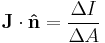
Product form Starting from 
since L = 0 when p and r are parallel or antiparallel, and is a maximum when perpendicular, so that the only component of p which contributes to L is the tangential |p| sin θ, the magnitude of angular momentum L should be re-written as
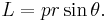
Since r, p and L form a right-hand triad, this leads to the vector form

- Elementary calculus
- The arithmetic operations are modified to the limiting cases of differentiation and integration. Equations can be expressed in these equivalent and alternative ways.
-
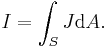
Current density Differential form 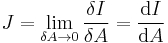
Integral form 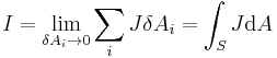
Alternatively for integral form

- Vector calculus
-
Current density Differential form 
Integral form 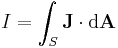
- Tensor analysis
- Vectors are rank-1 tensors. The formulae below are no more than the vector equations in the language of tensors.
-
Angular momentum Electric current density Differential form N/A 
Product/integral form Starting from 
the components are Li, rj, pi, where i, j, k are each dummy indices each taking values 1, 2, 3, using the identity from tensor analysis
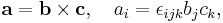
where εijk is the permutation/Levi-Cita tensor, leads to
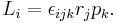
Using the Einstein summation convention, 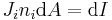
Multiple choice definitions
Sometimes there is still freedom within the chosen units system, to define one or more quantities in more than one way. The situation splits into two cases:
- Mutually exclusive definitions: There are a number of possible choices for a quantity to be defined in terms of others, but only one can be used and not the others. Choosing more than one of the exclusive equations for a definition leads to a contradiction – one equation might demand a quantity X to be defined in one way using another quantity Y, while another equation requires the reverse, Y be defined using X, but then another equation might falsify the use of both X and Y, and so on. The mutual disagreement makes it impossible to say which equation defines what quantity.
- Equivalent definitions: Defining equations which are equivalent and self-consistent with other equations and laws within the physical theory, simply written in different ways.
There are two possibilities for each case:
- One defining equation – one defined quantity: A defining equation is used to define a single quantity in terms of a number of others.
- One defining equation – a number of defined quantities: A defining equation is used to define a number of quantities in terms of a number of others. A single defining equation shouldn't contain one quantity defining all other quantities in the same equation, otherwise contradictions arise again. There is no definition of the defined quantities separately since they are defined by a single quantity in a single equation. Furthermore the defined quantities may have already been defined before, so if another quantity defines these in the same equation, there is a clash between definitions.
Contradictions can be avoided by defining quantities successively; the order in which quantities are defined must be accounted for. Examples spanning these instances occur in electromagnetism, and are given below.
- Examples
- Mutually exclusive definitions:
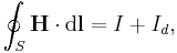
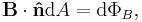
- The magnetic induction field B can be defined in terms of electric charge q or current I, and the Lorentz force (magnetic term) F experienced by the charge carriers due to the field,
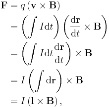
- where
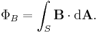
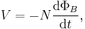
 is the change in position traversed by the charge carriers (assuming current is independent of position, if not so a line integral must be done along the path of current) or in terms of the magnetic flux ΦB through a surface S, where the area is used as a scalar A and vector:
  and
and  is a unit normal to A, either in differential form
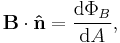
- or integral form,
- However, only one of the above equations can be used to define B for the following reason, given that A, r, v, and F have been defined elsewhere unambiguously (most likely mechanics and Euclidean geometry).
- If the force equation defines B, where q or I have been previously defined, then the flux equation defines ΦB, since B has been previously defined unambiguously. If the flux equation defines B, where ΦB, the force equation may be a defining equation for I or q. Notice the contradiction when B both equations define B simultaneously and when B is not a base quantity; the force equation demands that q or I be defined elsewhere while at the same time the flux equation demands that q or I be defined by the force equation, similarly the force equation requires ΦB to be defined by the flux equation, at the same time the flux equation demands that ΦB is defined elsewhere. For both equations to be used as definitions simultaneously, B must be a base quantity so that F and ΦB can be defined to stem from B unambiguously.
- Equivalent definitions:
- Another example is inductance L which has two equivalent equations to use as a definition (see the defined quantity tables of electromagnetism section).
- In terms of I and ΦB, the inductance is given by
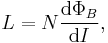
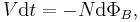
- in terms of I and induced emf V
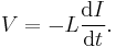
- These two are equivalent by Faraday's law of induction:
- substituting into the first definition for L
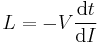
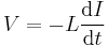
- and so they are not mutually exclusive.
- One defining equation – a number of defined quantities
- Notice that L cannot define I and ΦB simultaneously - this makes no sense. I, ΦB and V have most likely all been defined before as (ΦB given above in flux equation);
- where W = work done on charge q. Furthermore there is no definition of either I or ΦB separately – because L is defining them in the same equation.
- However, using the Lorentz force for the electromagnetic field
![\mathbf{F} = q \left [ \mathbf{E} %2B \left ( \mathbf{v} \times \mathbf{B} \right )\right ] ,\,\!](/2012-wikipedia_en_all_nopic_01_2012/I/819829044504bb3b4a906c5af86b8f9f.png)
- as a single defining equation for the electric field E and magnetic field B is allowed, since E and B are not only defined by one variable, but three; force F, velocity v and charge q. This is consistent with isolated definitions of E and B since E is defined using F and q:

- and B defined by F, v, and q, as given above.
Limitations of definitions
Definitions vs. functions: Defining quantities can vary as a function of parameters other than those in the definition. A defining equation only defines how calculate the defined quantity, it cannot describe how the quantity varies as a function of other parameters since the function would vary from one application to another.
- Examples
- Mass density ρ is defined using mass m and volume V by but can vary as a function of temperature T and pressure p, ρ = ρ(p, T)
- The angular frequency ω of wave propagation is defined using the frequency (or equivalently time period T) of the oscillation, as a function of wavenumber k, ω = ω(k). This is the dispersion relation for wave propagation.
- The coefficient of restitution for a object colliding is defined using the speeds of separation and and approach with respect to the collision point, but depends on the nature of the surfaces in question.
Definitions vs. theorems: There is a very important difference between defining equations and general or derived results, theorems or laws. Defining equations do not find out any information about a physical system, they simply re-state one measurement in terms of others. Results, theorems, and laws, on the other hand do provide meaningful information, if only a little, since they represent a calculation for a quantity given other properties of the system, and describe how the system behaves as variables are changed.
Examples
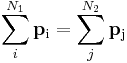
- An example was given above for Ampere's law. Another is the conservation of momentum for N1 initial particles having initial momenta pi where i = 1, 2 ... N1, and N2 final particles having final momenta pi (some particles may explode or adhere) where j = 1, 2 ... N2, the equation of conservation reads:
- Using the definition of momentum in terms of velocity:

- so that for each particle:
 and
and 
- the conservation equation can be written as
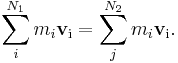
- It is identical to the previous version. No information is lost or gained by changing quantities when definitions are substituted, but the equation itself does give information about the system.
Pseudo-defining equations
Some equations, typically results from a derivation, contain quantities which may already be base quantities or have a definition, but be labelled in a different way with respect to the context of the result. These are not defining equations since they are results which apply to a physical situation – they are not quantity constructions, but can be used in the same way for calculations of the specific quantity within its scope of application.
- Examples
- Two examples in special relativity follow.
- Mass could be at rest or in motion (relativistic mass), relativistic mass can be pseudo-defined by

- where m0 = rest mass, m = relativistic mass and γ is the Lorentz factor.
- The invariant mass of a system could be pseudo-defined by the same equation as mass-momentum-energy invariance,
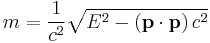
- where E = Total energy, p = Total 3-momentum of the system.
- Two examples in electromagnetism follow, neglecting relativistic effects for simplicity.
- Using SI units – not CGS or Gaussian which are fairly common in this field, the vacuum luminal speed c has the exact value c = 299 792 458 ms−1 (this in itself is the definition of the metre), and so does the vacuum permeability μ0 (another defined value, cannot be obtained from experiment), where μ0 = 4π × 10−7 Hm−1, so the value of the vacuum permittivity can be found from the pseudo-definition

- For a charged particle (of mass m and charge q) in a uniform magnetic field B, deflected by the field in a circular helical arc at velocity v and radius of curvature r, where the helical trajectory inclined at an angle θ to B, the magnetic force is the centripetal force, so the force F acting on the particle is;
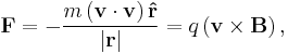
- reducing to scalar form and solving for |B||r|;
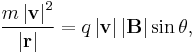
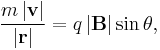
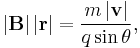
- serves as a pseudo-definition for the magnetic rigidity of the particle.[4]
Notice that these are all derived results from their respective theories – not proper definitions.
General derived quantities
Space
Important applied base units for space and time are below. Area and volume are of course derived from length, but included for completeness as they occur frequently in many derived quantities, in particular densities.
| (Common) Quantity name/s | (Common) Quantity symbol | SI unit | Dimension |
|---|---|---|---|
| (Spatial) position (vector) | r, R, a, d | m | [L] |
| Angular position, angle of rotation (can be treated as vector or scalar) | θ, θ | rad | dimensionless |
| Area, cross-section | A, S, Ω | m2 | [L]2 |
| Vector area (Magnitude of surface area, directed normal to tangential plane of surface) |  |
m2 | [L]2 |
| Volume | τ, V | m3 | [L]3 |
Densities, flows, gradients, and moments
Important and convenient derived quantities such as densities, fluxes, flows, currents are associated with many quantities. Sometimes different terms such as current density and flux density, rate, frequency and current, are used interchangeably in the same context, sometimes they are used uniqueley.
To clarify these effective template derived quantities, we let q be any quantity within some scope of context (not necessarily base quantities) and present in the table below some of the most commonly used symbols where applicable, their definitions, usage, SI units and SI dimensions - where [q] is the dimension of q.
For time derivatives, specific, molar, and flux densities of quantities there is no one symbol, nomenclature depends on subject, though time derivatives can be generally written using overdot notation. For generality we use qm, qn, and F respectively. No symbol is necessarily required for the gradient of a scalar field, since only the nabla/del operator ∇ or grad needs to be written. For spatial density, current, current density and flux, the notations are common from one context to another, differing only by a change in subscripts.
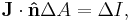
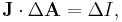
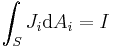
For current density,  is a unit vector in the direction of flow, i.e. tangent to a flowline. Notice the dot product with the unit normal for a surface, since the amount of current passing through the surface is reduced when the current is not normal to the area. Only the current passing perpendicular to the surface contributes to the current passing through the surface, no current passes in the (tangential) plane of the surface.
The calculus notations below can be used synonymously.
If X is a n-variable function 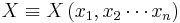 , then:
- Differential The differential n-space volume element is
 ,
,
- Integral: The multiple integral of X over the n-space volume is
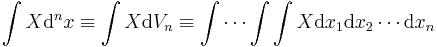 .
.
| Quantity | Typical symbols | Definition | Meaning, usage | Dimension |
|---|---|---|---|---|
| Quantity | q | q | Amount of a property | [q] |
| Rate of change of quantity, Time derivative |  |
 |
Rate of change of property with respect to time | [q] [T]−1 |
| Quantity spatial density | ρ = volume density (n = 3), σ = surface density (n = 2), λ = linear density (n = 1)
No common symbol for n-space density, here ρn is used. |
 |
Amount of property per unit n-space (length, area, volume or higher dimensions) |
[q][L]-n |
| Specific quantity | qm |  |
Amount of property per unit mass | [q][L]-n |
| Molar quantity | qn |  |
Amount of property per mole of substance | [q][L]-n |
| Quantity gradient (if q is a scalar field. |  |
Rate of change of property with respect to position | [q] [L]−1 | |
| Spectral quantity (for EM waves) | qv, qν, qλ | Two definitions are used, for frequency and wavelength:
|
Amount of property per unit wavelength or frequency. | [q][L]−1 (qλ) [q][T] (qν) |
| Flux, flow (synonymous) | ΦF, F | Two definitions are used; |
Flow of a property though a cross-section/surface boundary. | [q] [T]−1 [L]−2, [F] [L]2 |
| Flux density | F | 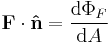 |
Flow of a property though a cross-section/surface boundary per unit cross-section/surface area | [F] |
| Current | i, I |  |
Rate of flow of property through a cross
section/ surface boundary |
[q] [T]−1 |
| Current density (sometimes called flux density in transport mechanics) | j, J | 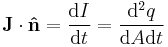 |
Rate of flow of property per unit cross-section/surface area | [q] [T]−1 [L]−2 |
| Moment of quantity | m, M | Two definitions can be used; q is a scalar: |
Quantity at position r has a moment about a point or axes, often relates to tendency of rotation or potential energy. | [q] [L] |


Physical quantities as coordinates over spaces of physical qualities (philosophy)
The meaning of the term physical quantity is generally well understood (everyone understands what is meant by the frequency of a periodic phenomenon, or the resistance of an electric wire). The term physical quantity does not imply a physically invariant quantity. Length for example is a physical quantity, yet it is variant under coordinate change in special and general relativity. The notion of physical quantities is so basic and intuitive in the realm of science, that it does not need to be explicitly spelled out or even mentioned. It is universally understood that scientists will (more often than not) deal with quantitative data, as opposed to qualitative data. Explicit mention and discussion of physical quantities is not part of any standard science program, and is more suited for a philosophy of science or philosophy program.
The notion of physical quantities is seldom used in physics, nor is it part of the standard physics vernacular. The idea is often misleading, as its name implies "a quantity that can be physically measured", yet is often incorrectly used to mean a physical invariant. Due to the rich complexity of physics, many different fields possess different physical invariants. There is no known physical invariant sacred in all possible fields of physics. Energy, space, momentum, torque, position, and length (just to name a few) are all found to be experimentally variant in some particular scale and system. Additionally, the notion that it is possible to measure "physical quantities" comes into question, particular in quantum field theory and normalization techniques. As infinities are produced by the theory, the actual “measurements” made are not really those of the physical universe (as we cannot measure infinities), they are those of the renormalization scheme which is expressly depended on our measurement scheme, coordinate system and metric system.
It is not always possible to define the distance between two points of any quality space, and this distance is —inside a given theoretical context— not uniquely defined. The notion of a distance, even in the context of quality space, relies on a concept of a metric space. Without a metric space, any notion of distance, physical or otherwise is undefined.
See also
References
- ^ http://www.bipm.org/utils/common/documents/jcgm/JCGM_200_2008.pdf
- ^ Joint Committee for Guides in Metrology (JCGM), International Vocabulary of Metrology, Basic and General Concepts and Associated Terms (VIM), III ed., Pavillon de Breteuil : JCGM 200:2008, 1.1 (on-line)
- ^ Fourier, Joseph. Théorie analytique de la chaleur, Firmin Didot, Paris, 1822. (In this book, Fourier introduces the concept of physical dimensions for the physical quantities.)
- ^ Electromagnetism (2nd edition), I.S. Grant, W.R. Phillips, Manchester Physics Series, 2008 ISBN 0 471 92712 0
Sources
- Cook, Alan H. The observational foundations of physics, Cambridge, 1994. ISBN 0-521-45597-
- Essential Principles of Physics, P.M. Whelan, M.J. Hodgeson, 2nd Edition, 1978, John Murray, ISBN 0 7195 3382 1
- Encyclopaedia of Physics, R.G. Lerner, G.L. Trigg, 2nd Edition, VHC Publishers, Hans Warlimont, Springer, 2005, pp 12–13
- Physics for Scientists and Engineers: With Modern Physics (6th Edition), P.A. Tipler, G. Mosca, W.H. Freeman and Co, 2008, 9-781429-202657